Each line is “time,value” separated by a comma. Use a consistent interval (e.g., hourly or daily) whenever possible.
Method 3: Upload a file
Best for: Real workflows when you have prepared CSV or TsFile files.
Supported file formats:
Format
Description
Typical use
CSV
Comma-separated text file with broad compatibility
Exports from Excel or databases
TsFile
Binary time-series format with high read/write efficiency
Exports from IoTDB and similar TSDBs
Steps:
Open the “Upload file” tab.
Click the upload area or drag the file into the dashed box to upload.
After upload, the system parses the file and shows basic info (row count, column names).
In “Assign column roles”, set each column as Time / Target / Covariate / Covariate (including future data) / Ignore.
Click “Confirm” to finish loading the data.
Three sample files are available at the bottom (values-only / timestamps / with covariates) to help you try the full flow quickly.
Add covariates (optional)
Covariates are external factors that influence the target variable, such as temperature, holidays, or promotions. Adding covariates can improve forecasting accuracy.
Depending on whether covariates include future data, the system supports three scenarios with increasing accuracy:
Scenario
Configuration
Description
Scenario 1
Target only
Forecast from historical target values only; suitable when no external factors are available.
Scenario 2
Target + covariates (no future data)
Use historical covariates to help modeling, but no covariate values are provided for the forecast horizon.
Scenario 3
Target + covariates (including future data)
Covariates are known for both history and future (e.g., holiday calendars), usually giving the best accuracy.
How to add covariates:
After loading the target data, expand ”+ Add covariates (optional)”.
Use the same three methods (draw / input / upload) to add covariate data.
Add multiple covariates; each one can be configured independently.
If covariates include future data, include them and mark the column as “Covariate (including future data)” so the model can leverage that information.
Forecast parameters
Click “Forecast parameters” in the upper-right to configure the following settings:
Parameter
Meaning
Range / Default
Recommendation
Steps
Number of time steps to forecast into the future
1–720, default 10
Set based on your needs
Start
Which row index to start forecasting from
Integer, defaults to the last row
Leave empty to use all historical data
If “Start” is set to a value smaller than the total rows, the system forecasts using the first “start” rows and compares the next “steps” rows with actual values for evaluation.
Run and view results
After data and parameters are ready, click the blue arrow button (→) to submit the forecasting task.
Quick try: three built-in examples
Three built-in examples are provided at the bottom to demonstrate the three input methods. Click one to load it instantly.
Example
Input method
Description
Forecast sales trend
Draw curve
Draw a historical sales curve and run a quick forecast.
Transformer oil temperature
Input data
Paste an industrial temperature series to validate the model.
Ice cream sales
Upload file
Upload a CSV with covariates (temperature) to try multivariate forecasting.
Each example comes with prefilled data. Click the example name to load it with no manual input, ideal for first-time users.
Model overview
Recommended default
Auto (Recommended)
Auto selection
TimechoAI’s in-house fusion model. The system automatically matches the best strategy based on your data, with no manual tuning needed.
Best for
Most industrial time-series forecasting scenarios. Recommended as the default choice.
Input limits
Request payload up to 20MB, maximum input length 11520, maximum output length 720, and up to 50 covariates.
Tsinghua University THUML
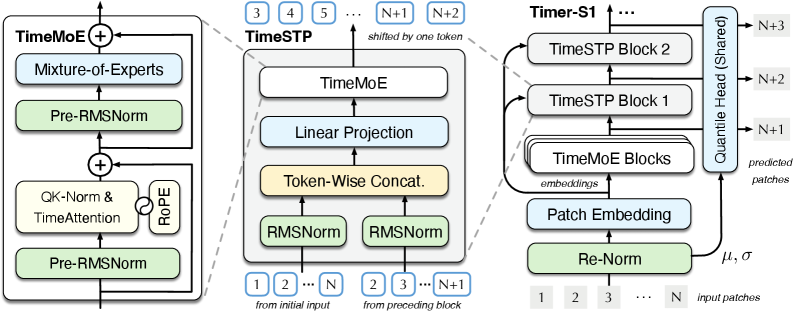
Timer-3.5
High accuracy
A TimechoAI-optimized version of the open-source Timer foundation model from Tsinghua University’s data team, with stronger accuracy and industrial data adaptability. It can provide forecasts under different confidence levels and generate future trends step by step based on the forecast horizon, making it a better fit for accuracy-sensitive tasks.
Best for
Scenarios with higher accuracy requirements.
Input limits
Request payload up to 20MB, maximum input length 11520, maximum output length 720. Covariate input is not currently supported.
Tsinghua University THUML
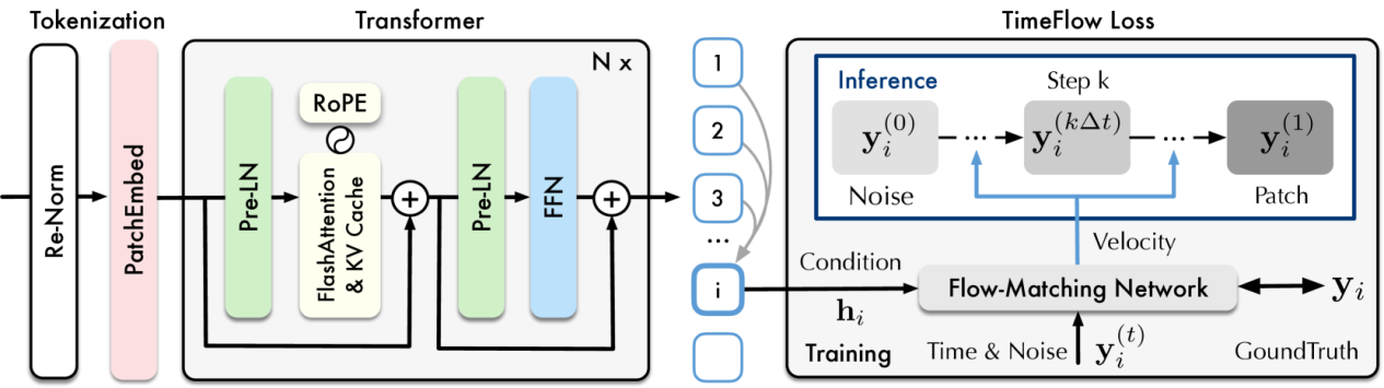
Timer-3.0
Stable
A stable, optimized version of the Timer series with good generalization and industrial adaptability. It combines multiple plausible future trajectories into the final forecast, offering balanced performance when data patterns vary and stability matters.
Best for
Scenarios that prioritize stability or need consistency with historical versions.
Input limits
Request payload up to 20MB, maximum input length 2880, maximum output length 720. Covariate input is not currently supported.
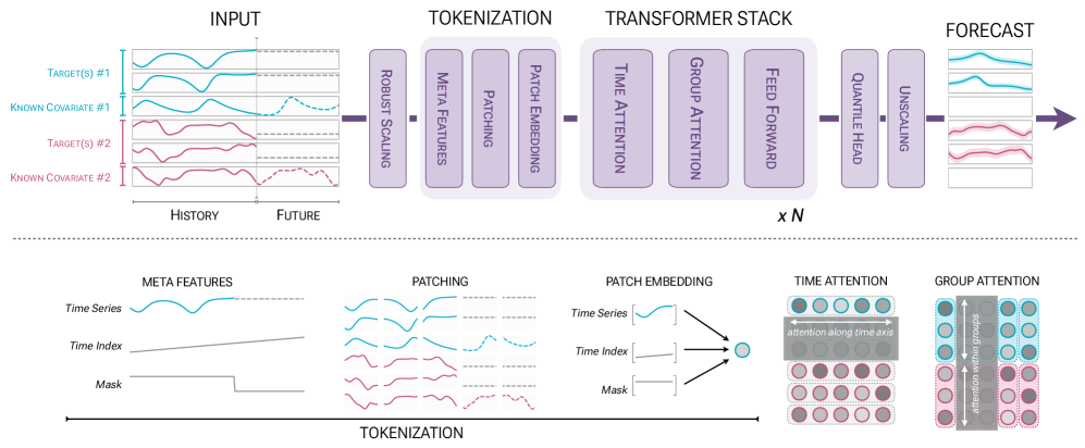
Amazon Science
Chronos-2
Covariates
Amazon’s open-source time-series foundation model with strong zero-shot forecasting capability and support for multiple covariates. It can use the target series, related series, and external variables together to produce multi-step forecasts, making it suitable when business factors should be considered alongside historical trends.
Best for
Benchmark comparisons, exploratory forecasting, and scenarios that require covariate-based forecasting.
Input limits
Request payload up to 20MB, maximum input length 8192, maximum output length 720, and up to 50 covariates.
Traditional statistical model
AutoARIMA
Baseline
Classic statistical model with automatic parameter search.
Best for
Smaller datasets with clear trends or seasonality; also useful as a baseline.
Input limits
Request payload up to 20MB, maximum input length 2880, maximum output length 720. Covariate input is not currently supported.
Traditional statistical model
Holt-Winters
Lightweight
Traditional exponential smoothing model designed for trend and seasonal data. Lightweight and interpretable.
Best for
Forecasting with strong periodic patterns or limited compute resources.
Input limits
Request payload up to 20MB, maximum input length 2880, maximum output length 720. Covariate input is not currently supported.
Tip: If you’re unsure which model to choose, use Auto. The system will select the optimal forecasting approach for your data. For larger-scale data ingestion, consider a private deployment. Contact us for details.
FAQ
Q: What if column roles are auto-detected incorrectly after upload?
In “Assign column roles”, set each column to the correct role (Time / Target / Covariate / Ignore), then click “Confirm”.
Q: Can I use covariates without future data?
Yes. Mark the column as “Covariate” (instead of “Covariate (including future data)”). The system will use only historical covariate values. Accuracy may be slightly lower than with future data, but typically better than using none.
Q: Can I edit after drawing a curve?
Yes. Click “Reset” to redraw, or switch to “Input data” to edit values directly.